2.1.1 Average Rates of Change: Slopes of
         Linear Equations

In the introduction to this chapter we mentioned Malthus's belief in linear growth of the world's food supply. Probably, linear functions are familiar from your previous study of mathematics. You associate them with linear equations, such as,

${\displaystyle y=mx+b}$,

where \(x\) is the input (also called the independent variable), \(y\) is the output (also called the dependent variable), \(m\) is the slope, and \(b\) is the \(y\)-intercept (i.e., the value of the function when $x=0$). For linear equations we know that

slope = rise run.

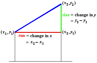
Figure 1   Slope equals rise over run

That is, the slope of the line connecting two points \((x_1,y_1)\) and \((x_2,y_2)\) is the ratio described by each of the following expressions — all of which say the same thing (see Figure 1):

• rise over run

• change in \(y\) over change in \(x\)

• $y_2-y_1$ over $x_2-x_1$

Lines are very special curves. The essence of linearity is that the slope of a line does not depend on which two points are selected for the computation. The ratio of rise to run is the same no matter where you start and no matter how long the run is or in which direction.

Activity 1

1. Devise a method for drawing a line with slope 2. Pick a point you want the line to go through. Then decide how you will find a second point on the line. Draw your line, and use two other points on it to check its slope.

2. Repeat for slope $-\frac{1}{2}$. Do you notice anything special about the relationship between this line and the one in part (a)?

Comment on Activity 1

Checkpoint 1