Chapter 2
Models of Growth: Rates of Change
 2.6
Logarithms and Representation of Data
Exercises
![]() The data in each of the following tables (Exercises 1-4) approximately fit either an exponential function or a power function. In each case, decide which, and find a formula that fits the data. Each formula should have one of the forms \(y=c b^t\), \(y=c e^{kt}\), or \(y=c t^k\), with explicit values for the constants. You may use the Plot Data tool to decide which formula to try, or you can do these exercises entirely with the numeric calculator. The Plot Data tool has the data for Exercise 1. You can edit the data entry for Exercises 2, 3, 4.
The data in each of the following tables (Exercises 1-4) approximately fit either an exponential function or a power function. In each case, decide which, and find a formula that fits the data. Each formula should have one of the forms \(y=c b^t\), \(y=c e^{kt}\), or \(y=c t^k\), with explicit values for the constants. You may use the Plot Data tool to decide which formula to try, or you can do these exercises entirely with the numeric calculator. The Plot Data tool has the data for Exercise 1. You can edit the data entry for Exercises 2, 3, 4.
| 1. | \(t\) |
\(y\) |
2. | \(t\) |
\(y\) |
||
|---|---|---|---|---|---|---|---|
5 |
14.855 |
5 |
4.452 |
||||
10 |
20.292 |
10 |
7.339 |
||||
15 |
24.354 |
15 |
12.101 |
||||
20 |
27.720 |
20 |
19.950 |
||||
25 |
30.648 |
25 |
32.893 |
| 3. | \(t\) |
\(y\) |
4. | \(t\) |
\(y\) |
||
|---|---|---|---|---|---|---|---|
1 |
24.7 |
1 |
25.0 |
||||
5 |
17.2 |
5 |
7.5 |
||||
10 |
11.0 |
10 |
4.4 |
||||
20 |
4.5 |
20 |
2.6 |
||||
35 |
1.2 |
35 |
1.7 |
||||
50 |
0.3 |
50 |
1.3 |
-
The data in Table E1 are graphed in Figures E1, E2, and E3, in Cartesian, semilog, and log-log plots, not necessarily in that order.
- Decide whether the data come from a linear function, a power function, an exponential function, or none of these.
Estimate \(f(2)\).
Estimate \(f\,' (2)\).
-
The data in Table E2 are graphed in Figures E4, E5, and E6, in Cartesian, semilog, and log-log plots, not necessarily in that order.
-
Decide whether the data come from a linear function, a power function, an exponential function, or none of these.
- Find a formula for \(f\) as a function of \(t\) .
-

Table E3 shows the population of Mexico for each of the years 1980 through 1986.Table E3 Population
of MexicoYear Population
(millions)198067.38198169.13198270.93198372.77198474.66198576.60198678.59
- Find an exponential function that approximately fits these data.
- By what percentage did the population grow each year?
- What does your formula predict for the population in 2010? (The actual population in 2010 was about 111 million.)
- Find an exponential function that approximately fits these data.

Table E4 shows the U.S. Census data for the Houston, Texas, primary statistical metropolitan area over a period of 130 years.Table E4 Houston
area populationYear Population 185018,632186035,441187048,986188071,316189086,2241900134,6001910185,6541920272,4751930455,5701940646,8691950947,50019601,430,39419701,999,31619802,905,34419903,731,01420004,671,23020105,946,800
- Show that the historic population data for Houston are approximated by an exponential function, and find a formula for the function.
- According to your model formula, how long does it take for Houston's population to double?
- If the growth pattern continues into the future, what will the Houston area population be in 2050?
- Show that the historic population data for Houston are approximated by an exponential function, and find a formula for the function.
|
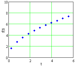 Figure E1 A plot of data in Table E1 |
||||||||||||||||||||||||
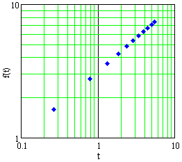 Figure E2 A plot of data in Table E1 |
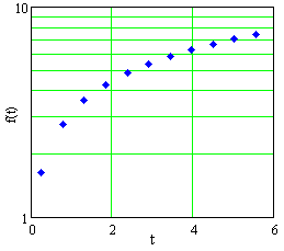 Figure E3 A plot of data in Table E1 |
|
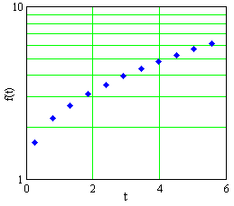 Figure E4 A plot of data in Table E2 |
||||||||||||||||||||||||
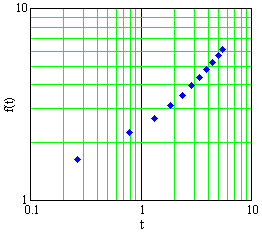 Figure E5 A plot of data in Table E2 |
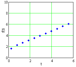 Figure E6 A plot of data in Table E2 |

