8.2.5 Calculation of the Vertical Moment and of \(\bar{y}\)

We return to our aircraft mobile scenario to discuss the \(y\)-coordinate of the center of mass, \(\bar{y}\). We do not need to know \(\bar{y}\) if we want the cutout to hang vertically - all we have to do is attach the string near the top edge along the line \(x = \bar{x}\). On the other hand, we would need to know \(\bar{y}\) if we want to balance the cutout in a horizontal position.

We have already done most - not all - of the hard work of figuring out how to calculate \(\bar{y}\). Instead of thinking of the \(y\)-axis as a balance line, we need to think now of the \(x\)-axis in this way. We already know a formula for the mass \(m\) of our cardboard shape. Whatever \(\bar{x}\) and \(\bar{y}\) turn out to be, if we placed a point mass \(m\) at the point \((\bar{x}, -\bar{y})\) and connected it to the cutout with a very light rod, the combined figure should balance at the point \((\bar{x},0)\), i.e., along the \(x\)-axis. Thus, just as was the case with \(\bar{x}\), we have

where \(M_x\) is the moment with respect to the \(x\)-axis. The question is, how do we calculate \(M_x\)?

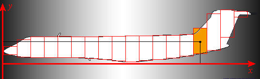
In Figure 6 we repeat the picture highlighting the \(k\)th rectangle. Observe that \(\bar{y}_k\), the \(y\)-coordinate of the center of mass of the typical rectangle, has already been identified. In general, if we know \(y\)-coordinates for the top and bottom of the typical rectangle, the average of those coordinates will be \(\bar{y}_k\). Since we may consider the mass \(\theta \delta \,h(\bar{x}_k) \Delta x\) of the \(k\)th rectangle to be concentrated at \((\bar{x}_k, \bar{y}_k)\), the contribution of this rectangle to \(M_x\) is approximately \(y_k\,\theta \delta \,h(\bar{x}_k) \Delta x\). Thus

Notice the similarity between this approximate equation and the corresponding formula for the horizontal moment,

As the number \(n\) of subintervals becomes large, the right-hand side of

approaches \(M_x\). That right-hand side also approaches an integral, but to say what integral, we need some more notation.

Let us suppose that the top edge of the airplane shape is the graph of a function \(y=f(x)\), and the bottom edge is the graph of another function \(y=g(x)\). (This is not strictly possible with our airplane shape, because there is one place where the top edge doubles back on itself, as well as two where the bottom edge does so. We will ignore this complication; we could easily smooth off these rough edges without changing the center of mass much.) Then our height function \(h(x)\) is \(f(x)-g(x)\). Furthermore, we can express the \(y\)-coordinate of the center of mass of each rectangle in our subdivision in terms of \(f\) and \(g\):

In this notation,

becomes

In terms of the functions \(f\) and \(g\), it is clear how each component of the moment approximation depends on \(x\), so it is now clear what integral is being approached by the sums - and therefore what integral represents \(M_x\):

This equation contains a lot of symbols, but it says something familiar. First, there are the factors of \(\theta\) and \(\delta\) that will cancel with the corresponding factors in the mass calculation. Second, the integral has factors for the moment arm of each thin rectangle,

for the height of each rectangle,

and for the width, \(dx\), of each rectangle. The calculation of \(\bar{y}\) therefore fits into the same pattern we saw for \(\bar{x}\):

Checkpoint 4

We can no more complete the calculation of \(\bar{y}\) for our airplane shape than we could of \(\bar{x}\), and for the same reason: We don't know formulas for the functions \(f\) and \(g\). Thus, to illustrate the use of the formula from Checkpoint 4 for actually computing a \(\bar{y}\), we return to the shape you considered in Checkpoint 2 and Checkpoint 3.

Example 1

Find \(\bar{y}\) for the region of the \(xy\)-plane bounded above by \(y=\sqrt{x}\), below by the \(x\)-axis, and on the right by the line \(x=1\).

Solution   The upper boundary curve is \(f(x)=\sqrt{x}\), and the lower boundary curve is \(g(x)=0\), both defined for \(x\) running from \(0\) to \(1\). When \(g(x)=0\), our formula takes the simpler form

Thus

You found in Checkpoint 2 that the area of the region is \(2/3\) - equivalently, the mass is \(\frac{2 \theta \delta}{3}\) - so \(\bar{y} = 3/8\). 

Try this at home: If you can send a file to a printer, click here for a printable copy of the region in Example 1 from which you can make your own balance experiment.