5.2.1 A Numerical Solution for the Velocity-Squared Model

We continue our study of the Velocity-Squared Model for the velocity \(v\) of falling raindrops with diameters greater than \(0.05\) inches. As we noted in Section 5.1, we are considering an initial value problem of the form

where \(c\) is a constant that depends on the diameter of the raindrop.

In Section 5.1, we stated -- with no evidence whatsoever -- a symbolic solution of this problem. We won't be able to derive this solution until later, but here we show how to obtain an elementary numerical solution.

Our goal is to estimate values of \(v\) at a sequence of equally spaced times. Select a time step \(\Delta t\) and use it to generate a sequence of time values

and so on.

Our estimated velocity values at these times will be denoted by \(v_0,\,v_1,\,v_2, ...\). Our method for estimating the velocity values will be recursive, i.e., \(v_k\) will be calculated from the preceding \(v_{k-1}\) for each \(k=1,2,...\).

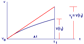
How do we obtain \(v_1\) from \(v_0=0\), the initial velocity? We answer this in a geometric fashion by considering the (unknown) graph of velocity versus time in the \((t,v)\)-plane. Figure 1 shows the first step.

Note 1 – Orientation

Our desired next velocity value, \(v(t_1)\), is the length of a vertical line segment to the solution graph at time \(t_1\). However, since the value of \(v(t_1)\) is not known to us, we will estimate its value by drawing the tangent line to the graph at \(t = t_0\). We follow this tangent line to the point on the tangent line with \(t=t_1\), and we call the \(v\)-coordinate of that point \(v_1\).

Now, we can compute \(v_1\). Since we start at \(v=v_0=0\), the value is just the rise along the line. We know

so \(v_1=\)slope \(\times\,\Delta t\). But we know the value of the slope: \(g-c\,{v_0}^2\). So

We use the same method to approximate \(v_2\):

And so on for \(v_3\), \(v_4\), etc.

That is, to get from each \(v\) to the next one, we need to compute a rise - a vertical change from one point on the solution curve to another. Because we have no way to do that exactly, we compute the rise to the tangent line as slope times run:

Activity 1

Explore the approximation technique just described.