Section 5-3-5

Chapter 5
Modeling with Differential Equations

5.3 Periodic Motion

5.3.5 Derivatives of Sine and Cosine 1: Examination

To model repeating phenomena by sine and cosine functions, we need to know the rates of change of these two functions. Thus, it is time to calculate those derivatives.

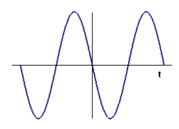
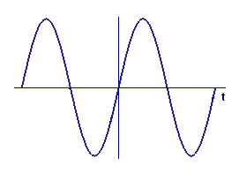
We start with some pictorial evidence of what to look for. In Figure 5, we show a graph of the sine function and in Figure 6 a graph of an approximate derivative, calculated as

approximate derivative of

\sin (t) = \frac{\sin (t + 0.001) - \sin (t)}{0.001} .


Figure 5 The sine function		Figure 6 Approximate derivative of $\sin t$

Activity 5

Sketch Figures 5 and 6 on a piece of paper. Or, if you have a printer available, click on either figure, and print the pop-up page.
On your copy of Figure 5 label $0$ and $1$ on the vertical axis. Indicate the $t$ values of the points where the graph intersects the horizontal axis. Label the approximate position of $1$ on the horizontal axis.
The scales are the same for Figure 6 -- label it also.
Why does the expression

$\frac{\sin (t + 0.001) - \sin (t)}{0.001}$

approximate the derivative of $\sin t$?
What do you see in the graph in Figure 6? What function do you think is the derivative of $\sin t$?

Comment on Activity 5

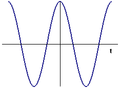
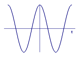
In Figures 7 and 8, we do the same thing with the cosine function that we just did with the sine function. The image in Figure 8 is the graph of

approximate derivative of

\cos (t) = \frac{\cos (t + 0.001) - \cos (t)}{0.001} .


Figure 7 The cosine function		Figure 8 Approximate derivative of $\cos t$

Checkpoint 5

Contents for Chapter 5


Figure 5 The sine function		Figure 6 Approximate derivative of \(\sin t\)


Figure 7 The cosine function		Figure 8 Approximate derivative of \(\cos t\)

Chapter 5 Modeling with Differential Equations

5.3 Periodic Motion

Chapter 5
Modeling with Differential Equations