8.2.3 Calculation of the Horizontal Moment

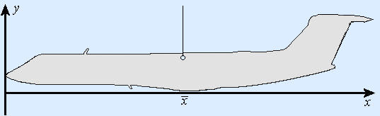
The \(x\)-coordinate \(\bar{x}\) is the location along the \(x\)-axis where, if you threaded through a hole in the edge of the cutout, it would balance from the thread (see Figure 4). As in the one-dimensional case, the horizontal moment of the figure is the product of \(\bar{x}\) and the mass. Because \(\bar{x}\) is measured from the \(y\)-axis, this moment is called the moment with respect to the \(y\)-axis and is denoted \(M_y\). Thus, for a point mass \(m\) with \(x\)-coordinate \(\bar{x}\), \(M_y = \bar{x} m\). Our balance condition for \(\bar{x}\) is that the moment with respect to the \(y\)-axis of a point mass \(m\) with \(x\)-coordinate \(\bar{x}\) equals the moment \(M_y\) of the whole cutout.

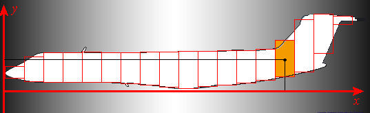
Now we consider the problem of calculating \(M_y\). In Figure 5 we have selected and shaded a typical approximating rectangle and called it the \(k\)th rectangle. (It happens that \(k\) is \(15\) for this discussion.) It is easy to locate the center of mass of this rectangle: It must be at the geometric center. And it is easy to determine the coordinates \(( \bar{x}_k , \bar{y}_k)\) of that center: \(\bar{x}_k\) is the average of \(x_{k-1}\) and \(x_k\), and \(\bar{y}_k\) is the average of the \(y\)-coordinates of the top and bottom of the rectangle. We also know the mass of this rectangle:

height \(\times\) width \(\times\) thickness \(\times\) density.

or \(h(\bar{x}_k)(\Delta x) \theta \delta\), at least approximately. Thus we can approximate the moment for this rectangle by multiplying this mass by the moment arm, the distance of the center of mass from the \(y\)-axis, which is just \(\bar{x}_k\).

Now we can sum the moment contributions from all \(n\) rectangles to find that

This too is an approximating sum for an integral, but not an integral of \(h\). Rather, after we factor out the constant factors, \(\theta\) and \(\delta\), we have a sum of the form

where the new function \(w\) is defined by \(w(x)=x\,h(x)\). As the number \(n\) of subdivisions increases, the approximating sum (including the constant factors of \(\theta\) and \(\delta\)) gets closer to the moment we seek and also to the integral it approximates, so we conclude that \(M_y\) is that integral: