Chapter 5
Modeling with Differential Equations
Project 2: The SIR Model of the Spread of Disease
- Introduction
- Variables, Parameters, and Assumptions
- The Model Equations
- Euler's Method for Systems
- Relating Model Parameters to Data
- The Contact Number
- Herd Immunity
- Summary Questions
The Model Equations
Let's see what these assumptions tell us about derivatives of our dependent variables.
The Susceptible Equation. Explain carefully how each component of the differential equation
follows from the assumptions. In particular,
- Why is the factor of \(I(t)\) present?
- Where did the negative sign come from?
Now explain how this equation leads to the following differential equation for \(s(t)\):
.The Recovered Equation. Explain how the corresponding differential equation for \(r(t)\),
,follows from one of the assumptions.
The Infected Equation. Explain why
.What assumption about the model does this reflect? Now explain carefully how each component of the equation
follows from what you have done thus far. In particular,
- Why are there two terms?
- Why is it reasonable that the rate of flow from the infected population to the recovered population should depend only on \(i(t)\)?
- Where did the minus sign come from?
Finally, we complete our model by giving each differential equation an initial condition. For this particular virus — Hong Kong flu in New York City in the late 1960's — hardly anyone was immune at the beginning of the epidemic, so almost everyone was susceptible. We will assume that there was a trace level of infection in the population, say, 10 people. Thus, our initial values for the population variables are
| \(S(0)\) | \(=7,900,000\), |
| \(I(0)\) | \(=10\), |
| \(R(0)\) | \(=0\). |
In terms of the scaled variables, these initial conditions are
| \(s(0)\) | \(=1\), |
| \(i(0)\) | \(=1.27\times10^{-6}\), |
| \(r(0)\) | \(=0\). |
(Note: The sum of our starting populations is not exactly \(N\), nor is the sum of our fractions exactly \(1\). The trace level of infection is so small that this won't make any difference.) Our complete model is
| \(\frac{ds}{dt}\) | \(=-b\,s(t)\,i(t)\), | \(s(0)\) | \(=1\), |
| \(\frac{di}{dt}\) | \(=b\,s(t)\,i(t)-k\,i(t)\), | \(i(0)\) | \(=1.27\times10^{-6}\), |
| \(\frac{dr}{dt}\) | \(=k\,i(t)\), | \(r(0)\) | \(=0\). |
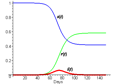
We don't know values for the parameters \(b\) and \(k\) yet, but we can estimate them, and then adjust them as necessary to fit the excess death data. We have already estimated the average period of infectiousness at three days, so that would suggest \(k = 1/3\). If we guess that each infected would make a possibly infecting contact every two days, then \(b\) would be \(1/2\). We emphasize that this is just a guess. The following plot shows the solution curves for these choices of \(b\) and \(k\).
 |
| Figure 2 |
In Steps 1 and 2 on the previous page, you recorded your ideas about what the solution functions should look like. How do those ideas compare with the figure above? In particular,
- What do you think about the relatively low level of infection at the peak of the epidemic?
- Can you see how a low peak level of infection can nevertheless lead to more than half the population getting sick? Explain.


