Chapter 5
Modeling with Differential Equations
Project 2: The SIR Model of the Spread of Disease
- Introduction
- Variables, Parameters, and Assumptions
- The Model Equations
- Euler's Method for Systems
- Relating Model Parameters to Data
- The Contact Number
- Herd Immunity
- Summary Questions
Relating Model Parameters to Data
The infectious period for Hong Kong Flu is known to average about three days, so our estimate of \(k = 1/3\) is probably not far off. However, our estimate of \(b\) was nothing but a guess. Furthermore, a good estimate of the "mixing rate" of the population would surely depend on many characteristics of the population, such as density. Here we experiment with the effects of these parameters on the solutions, and then try to find values that are in agreement with the excess deaths data from New York City. We focus our experimentation on the infected-fraction, \(i(t)\), since that function tells us about the progress of the epidemic.
First let's experiment with changes in \(b\). Keep \(k\) fixed at \(1/3\), and plot the graph of \(i(t)\) with several different values of \(b\) between \(0.5\) and \(2.0\). Describe how these changes affect the graph of \(i(t)\). Stay alert for automatic changes in the vertical scale.
Explain briefly why the changes you see are reasonable from your intuitive understanding of the epidemic model.
Now let's experiment with changes in \(k\). Return \(b\) to \(1/2\), and experiment with different values of \(k\) between \(0.1\) and \(0.6\). Describe the changes you see in the graph of \(i(t)\). Again, be alert for automatic changes in the vertical scale.
Explain the changes you see in terms of your intuitive understanding of the model.
There is a change in the character of the graph of \(i(t)\) near one end of the suggested range, \(0.1\) to \(0.6\), for \(k\). What is the change, and where does it occur?
Use the infected-fraction differential equation
to explain how you could have predicted in advance the value of \(k\) at which the character of the graph of \(i(t)\) changed.
-
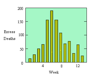
Now let's compare our model with the data. Recall that these were the numbers of deaths each week that could be attributed to the flu epidemic. If we assume that the fraction of deaths among infected individuals is constant, then the number of deaths per week should be roughly proportional to the number of infecteds in some earlier week. We repeat the graph of the data, along with the graph of \(i(t)\) with \(k = 1/3\) and \(b = 6/10\) (Figure 3). Does the model seem reasonable or not? Explain your conclusion.


Figure 1 (repeated) Figure 3


